Physical Simulation: Eulerian Fluid Simulation

Overview

Material Derivatives: Lagrangian v.s. Eulerian

We define material derivative as

$$\frac{\text{D}}{\text{D}t} := \frac{\partial}{\partial t} + \textbf{u} \cdot \nabla$$

E.g.,

$$\frac{\text{D} T}{\text{D}t} := \frac{\partial T}{\partial t} + \textbf{u} \cdot \nabla T \\ \ \\ \frac{\text{D} \textbf{u}_{x}}{\text{D} t} := \frac{\partial \textbf{u}_{x}}{\partial t} + \textbf{u} \cdot \nabla \textbf{u}_{x}$$

$\textbf{u}$: material (fluid) velocity. Many other names: Advective/Lagrangian/particle derivative.

Intuitively, change of physical quantity on a piece of material =

• change due to time $\frac{\partial}{\partial t}$(Eulerian)
• change due to material movement $\textbf{u} \cdot \nabla$

(Incompressible) Navier-Stokes equations

$$\rho \frac{\text{D} \textbf{u}}{\text{D} t} = - \nabla p + \mu \nabla^{2} \textbf{u} + \rho \text{g} \\ \textbf{or} \\ \frac{\text{D} \textbf{u}}{\text{D} t} = - \frac{1}{\rho} \nabla p + \nu \nabla^{2} \textbf{u} + \text{g} \\ \ \\ \nabla \cdot \textbf{u} = 0$$

where $\mu$: dynamic viscosity; $\nu = \frac{\mu}{\rho}$: kinematic viscosity.

Operator splitting

$$\frac{\text{D} \textbf{u}}{\text{D} t} = - \frac{1}{\rho} \nabla p + \nu \nabla^{2} \textbf{u} + \text{g} ,\quad \nabla \cdot \textbf{u} = 0$$

Split the euqations above into three parts:

$$\frac{\text{D} \textbf{u}}{\text{D} t} = 0, \quad \frac{\text{D} \alpha}{\text{D} t} = 0 \quad \textbf{(advection)} \\ \ \\ \frac{\partial \textbf{u}}{\partial t} = \text{g} \quad \text{(external forces, optional)} \\ \ \\ \frac{\partial \textbf{u}}{\partial t} = - \frac{1}{\rho} \nabla p \quad \text{s.t.} \quad \nabla \cdot \textbf{u} = 0 \quad \textbf{(projection)}$$

$\alpha$: any physical property (temperature, color, smoke density etc.)

Eulerian fluid simulation cycle

Time discretization with splitting: for each time step,

1. Advection: “move” the fluid field. Solve $\textbf{u}^{*}$ using $\textbf{u}^{t}$

   $$\frac{\text{D} \textbf{u}}{\text{D} t} = 0, \quad \frac{\text{D} \alpha}{\text{D} t} = 0$$

2. External forces (optional): evaluate $\textbf{u}^{*}$ using $\textbf{u}^{}$

   $$\frac{\partial \textbf{u}}{\partial t} = \text{g}$$

3. Projection: make velocity field $\textbf{u}^{t+1}$ divergence-free based on $\textbf{u}^{**}$

   $$\frac{\partial \textbf{u}}{\partial t} = - \frac{1}{\rho} \nabla p \quad \text{s.t.} \quad \nabla \cdot \textbf{u}^{t+1} = 0$$

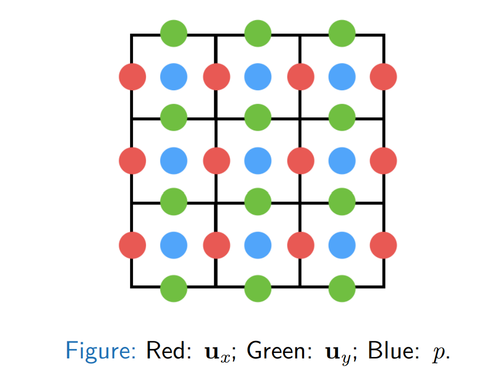
Grid

Spatial discretization using cell-centered grids or staggered grids

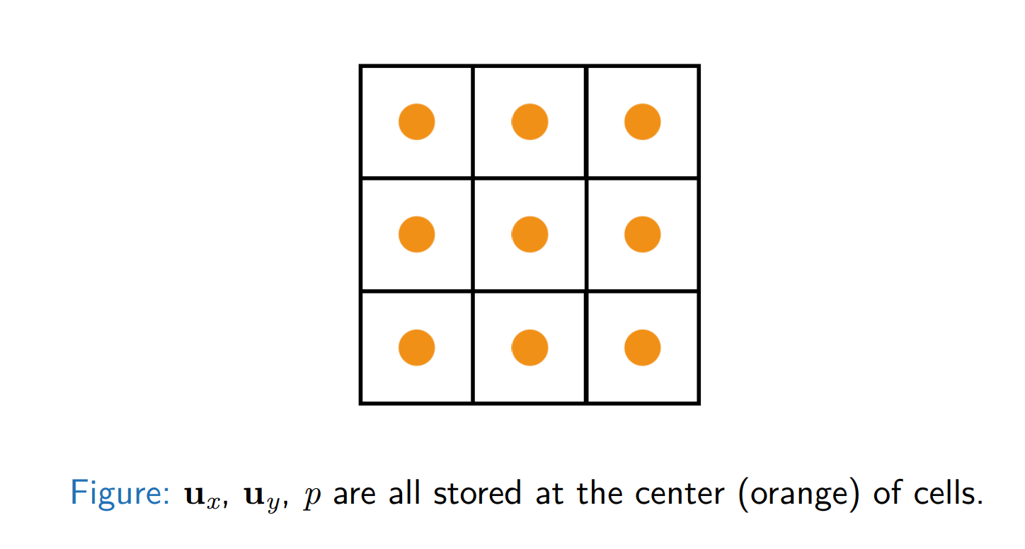
v.s.

And for any point within a grid, just use bilinear interpolation. As it’s an obvious and straightforward method, we move on

Advection

Advection schemes

A trade-off between numerical viscosity, stability, performance and complexity:

• Semi-Lagrangian advection
• MacCormack/BFECC
• BiMocq
• Particle advection (PIC/FLIP/APIC/PolyPIC)
• …

Semi-Lagrangian advection

1. To find a fluid value at grid point $\vec{x}{G}$ at the new time step, we need to know where the fluid at $\vec{x}{G}$ was one time step ago, position $\vec{x}_{P}$, following the velocity field.

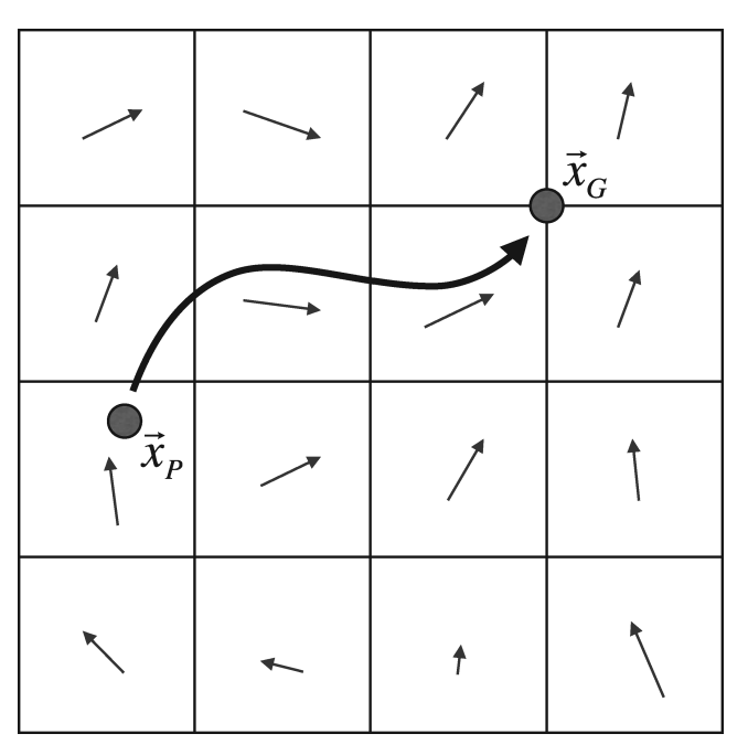
1. Now we use bilinear interpolation, our basic semi-Lagrangian formula, assuming the particle-tracing algorithm has tracked back to location $\vec{x}_{P}$ is $$q_{G}^{n+1} = \textbf{interpolate}(q_{G}^{n}, \vec{x}_{P})$$

Problem: The real trajectory of material parcels can be complex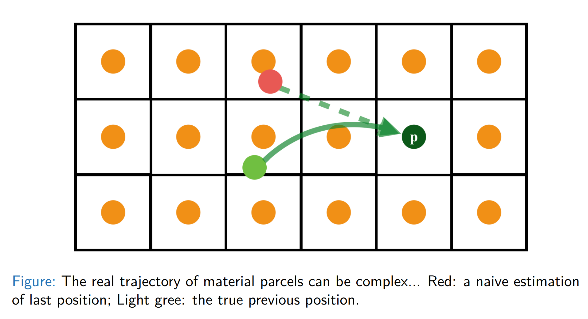

Solve the problem - Backtrace Method

Initial value problem (ODE): simply use explicit time integration schemes

• Forward Euler (“RK1”) $$q^{n+1} = q^{n} + \Delta t f(q^{n})$$
• Explicit Midpoint (“RK2”) $$q^{n+1/2} = q^{n} + \frac{1}{2} \Delta t f(q^{n}) \\ \\ q^{n+1} = q^{n} + \Delta t f(q^{n+1/2})$$
• RK3 $$k_{1} = f(q^{n}) \\ \\ k_{2} = f(q^{n} + \frac{1}{2} \Delta t k_{1}) \\ \\ k_{3} = f(q^{n} + \frac{3}{4} \Delta t k_{2}) \\ \\ q^{n+1} = q^{n} + \frac{2}{9} \Delta t k_{1} + \frac{3}{9} \Delta t k_{2} + \frac{4}{9} \Delta t k_{3}$$

BFECC and MacCormack advection schemes

BFECC: Back and Forth Error Compensation and Correction

• $\textbf{x}^{*} = \text{SL}(\textbf{x}, \Delta t)$
• $\textbf{x}^{*} = \text{SL}(\textbf{x}^{}, - \Delta t)$
• Estimate the error $\textbf{x}^{error} = \frac{1}{2}(\textbf{x}^{**} - \textbf{x})$
• Apply the error $\textbf{x}^{final} = \textbf{x}^{**} + \textbf{x}^{error}$

Be careful: need to prevent overshooting.

Projection

The project routine will subtract the pressure gradient from the intermediate velocity field $\vec{u}$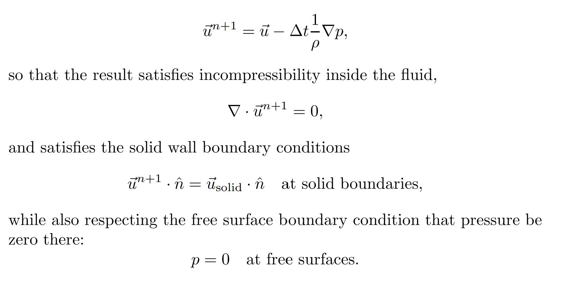

Actually after we combine the two euqations together we could easily get:

$$\nabla \cdot \nabla p = \frac{\rho}{\Delta t} \nabla \cdot \vec{u}$$

… which is Poisson’s equation

$$\nabla \cdot \nabla p = f \quad \textbf{or} \quad \Delta p = f.$$

If $f = 0$, the equation is called Laplace’s equation

Spatial discretization (2D)

Recall the euqation for $p$:

$$\nabla \cdot \nabla p = \frac{\rho}{\Delta t} \nabla \cdot \vec{u}$$

Discretize on a 2D grid:

$$(\textbf{Ap})_{i,j} = (\nabla \cdot \nabla p)_{i,j} = \frac{1}{\Delta x^{2}} (-4 p_{i,j} + p_{i+1,j} + p_{i-1,j} + p_{i,j-1} + p_{i,j+1}) \\ \ \\ (\textbf{b})_{i,j} = \frac{\rho}{\Delta t} \nabla \cdot \vec{u} = \frac{\rho}{\Delta t \Delta x} (\vec{u}_{i+1,j}^{x} - \vec{u}_{i,j}^{x} + \vec{u}_{i,j+1}^{y} - \vec{u}_{i,j}^{y})$$

Again, a linear system:

$$\textbf{A}_{nm \times nm} \textbf{p}_{nm} = \textbf{b}_{nm}$$

$n, m$: numbers of cells along the $x-$ and $y-$ axis

Solving large-scale linear systems

• Direct solvers (e.g. PARDISO)
• Iterative solvers
  • Gauss-Seidel
  • (Damped) Jacobi
  • (Preconditioned) Krylov-subspace solvers (e.g., conjugate gradients)

Extend reading

A great introduction to Eulerian fluid simulation: Fluid simulation for computer graphics by Robert Bridson
An Introduction to the Conjugate Gradient Method Without the Agonizing Pain
A introduction to Conjugate Gradient Method in Chinese