I come across this talk the other day and find the paper’s result astonishingly impressive. This DeepMind project can be found here.
- Paper: arxiv.org/abs/2002.09405
- Code & Datasets: https://github.com/deepmind/deepmind-research/tree/master/learning_to_simulate
High Level Overview - Simulation as Message-Passing on a Graph
First Step - Construct the graph
Particles within a particular small distance from each other are given edges so particles only interact with their immediate neighbors.
Features are assigned to each of the nodes and each of the edges
- Nodes: Its mass, its other material properties, velocities of previous five time steps ……
- Edges: The distance between the two particles that are interacting, the spring constant, ……
Second Step - Message passing
- Nodes in the graph send massages to the neighbors they’re connected to
And then each node receives these signals from their neighbors
Update its representation of itself
Third Step - Decoder
- Takes these new updated states and turns them into acceleration vectors
- Final output of the network: to predict the acceleration of the particles in the current time step
Last Step
- Use these acceleration vectors and update the state
Modules
Encoder - Processor - Decoder
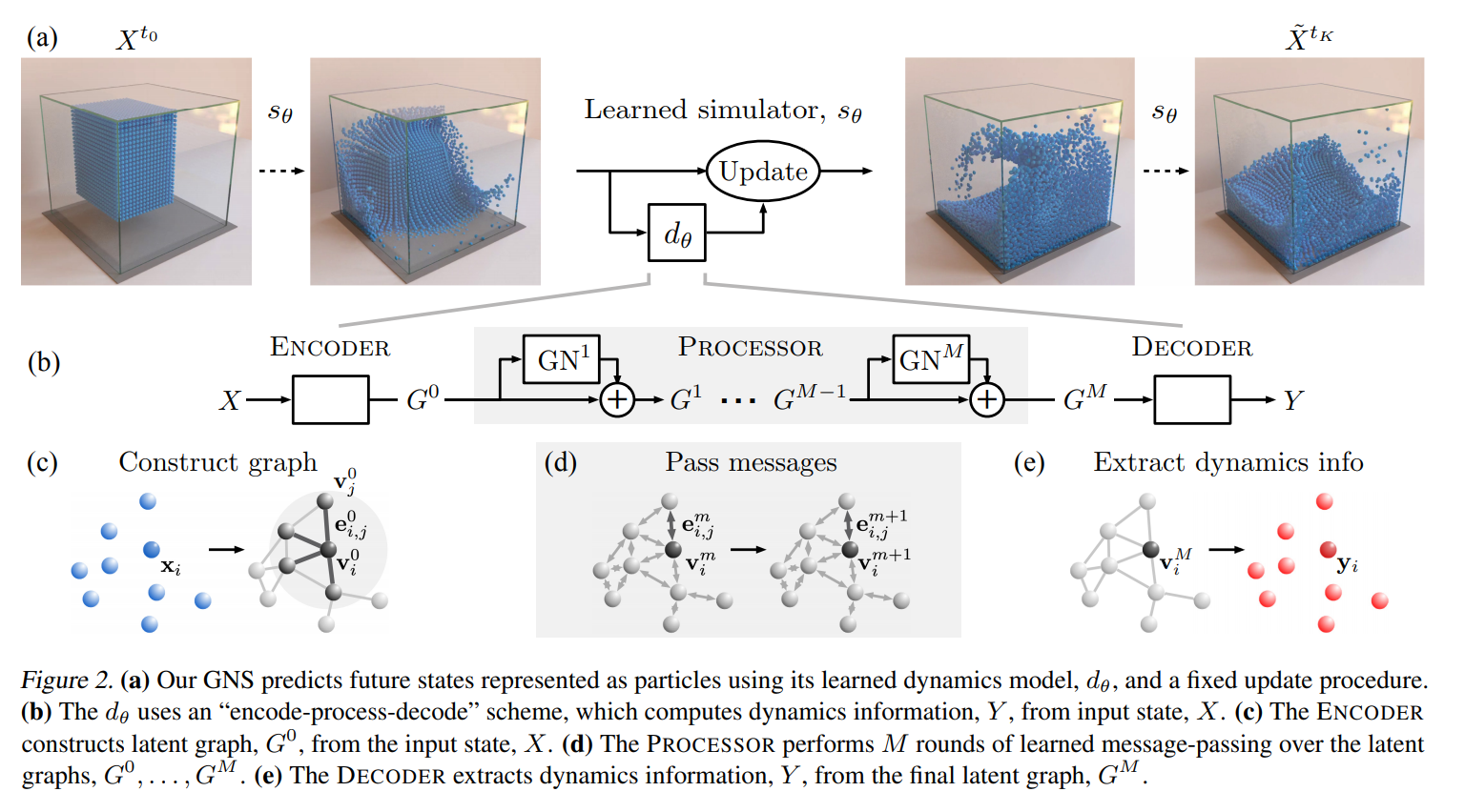
ENCODER
Responsible for constructing the graph
Initializing the node and edge features
One detail: they don’t just use the raw features, they first pass them through dedicated neural networks, that projects them into some new space that facilitates learning in the downstream tasks
At the end you have the initial embeddings
No interactions between particles has happened at this point
ENCODER definition:
The ENCODER: $\mathcal{X} \rightarrow \mathcal{G}$ embeds the particle based state representation, $X$, as a latent graph, $G^0 = ENCODER(X)$, where $G = (V, E, \mathbf{u}),\,\mathbf{v}i \in V$ and $\mathbf{e}{i, j} \in E$.
- The node embeddings, $\mathbf{v}_i = \varepsilon^v (\mathbf{x}_i)$, are learned functions of the particles’ states
- The edge embeddings, $\mathbf{e}{i,j} = \varepsilon^e (\mathbf{r}{i,j} )$, are learned functions of the pairwise properties of the corresponding particles
- The graph-level embedding, $\mathbf{u}$, can represent global properties such as gravity and magnetic fields
PROCESSOR
The number of graph network layers you have determines how far each message can propagate: e.g. three layers means you can go three hops away from a node
At the end of the process you have updated embeddings for each of the nodes that now takes into account its $m$-hop neighborhood where $m$ is the number of graph network layers used in the processor
PROCESSOR definition:
The PROCESSOR: $\mathcal{G} \rightarrow \mathcal{G}$ computes interactions among nodes via $M$ steps of learned message-passing, to generate a sequence of updated latent graphs, $\mathbf{G} = (G^1, …, G^M)$, where $G^{m+1} = GN^{m+1}(G^m)$. The final graph $G^M = PROCESSOR(G^0)$.
DECODER
Translate these updated embeddings into acceleration vectors
DECODER definition:
The DECODER: $\mathcal{G} \rightarrow \mathcal{Y}$ extracts dynamics information from the nodes of the final latent graph, $\mathbf{y}_i = \delta^v(\mathbf{v}_i^M)$
Why Graph Networks
How about regular neural networks
- First challenge: particles are going to interact with different neighborhood sizes
- Second challenge: neural networks/RNNs are not permutation-invariant, but real physical world is
Graph do a few useful things
- First: they encode what interact with what
- Second: they combine neighborhood information in a way that’s permutation-invariant
- Third: they are very data efficient because they have lots of examples that all share the same network parameters so all the particles are using the same model parameters