Physical Simulation: Smoothed Particle Hydrodynamics

Lagrange fluid simulation: Smoothed particle hydrodynamics

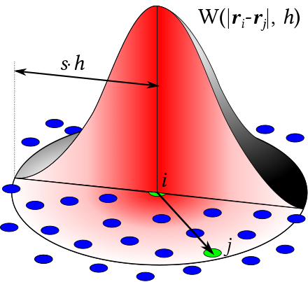
High-level idea: use particle carrying samples of physical quantities, and a kernel function $W$, to approximate continuous fields:

$A(\textbf{x}) = \sum_{i}{A_i\frac{m_i}{\rho_i}W\left( ||\textbf{x} - \textbf{x}_j||_2, h \right)}$

SPH particles and their kernel

Originally proposed for astrophysical problems
No meshes. Very suitable for free-surface flows!
Easy to understand intuitively: just imagine each particle is a small parcel of water (although strictly not the case)

Implementing SPH using the Equation of States (EOS)

Also know as Weakly Compressible SPH (WCSPH).

Momentum equation: ($\rho$: density; $B$: bulk modulus; $\gamma$: constant, usually $\sim 7$ )

$\frac{D\textbf{v}}{Dt} = -\frac{1}{\rho} \nabla p + \textbf{g} ,\ \ \ p = B\left( \left( \frac{\rho}{\rho_0} \right)^{\gamma} - 1 \right) \\ \ \\ \ \\ A(\textbf{x}) = \sum_{i}{A_i\frac{m_i}{\rho_i}W\left( ||\textbf{x} - \textbf{x}_j||_2, h \right)} ,\ \ \ \rho_i= \sum_j{ m_j W \left( ||\textbf{x} - \textbf{x}_j||_2, h \right)}$

Gradients in SPH

$A(\textbf{x}) = \sum_{i}{A_i\frac{m_i}{\rho_i}W\left( ||\textbf{x} - \textbf{x}_j||_2, h \right)} \\ \ \\ \nabla A_i = \rho_i \sum_{j} m_j \left( \frac{A_i}{\rho_i^2} + \frac{A_j}{\rho_j^2} \right) \nabla_{\textbf{x}_i} W\left( ||\textbf{x} - \textbf{x}_j||_2, h \right)$

Not really accurate
But at least symmetric and momentum conversing

Now we can compute $\nabla p_i$

SPH Simulation Cycle

For each particle $i$, compute $\rho_i= \sum_j{ m_j W \left( ||\textbf{x} - \textbf{x}_j||_2, h \right)}$
For each particle $i$, compute $\nabla p_i$ using the gradient operator
Symplectic Euler step:
$\textbf{v}_{t+1} = \textbf{v}_t + \Delta t \frac{D\textbf{v}}{Dt} \\ \textbf{x}_{t+1} = \textbf{x}_t + \Delta t \textbf{v}_{t+1}\$

Variants of SPH

Courant-Friedrichs-Lewy (CFL) condition

One upper bound of time step size:

$C = \frac{u \Delta t}{\Delta x} \le C_{max} \sim 1$

$C$: CFL number (Courant number, or simple the CFL)
$\Delta t$: time step
$\Delta x$: length interval (e.g. particle radius and grid size)
$u$: maximum (velocity)

Application: estimating allowed time step in (explicit) time integrations. Typical $C_{max}$ in graphics:

SPH: ~ 0.4
MPM: 0.3 ~ 1
FLIP fluid (smoke): 1 ~ 5+

Accelerating SPH: Neighborhood search

So far, per sub-step complexity of SPH is $O(n^2)$. This is too costly to be practical. In practice, people build spatial data structure such as voxel grid to accelerate neighborhood search. This reduces time complexity to $O(n)$.

Reference: Compact Hashing